Note: This blog post was initially written for the blog of Kensu.io, You can either read it here, or continue your reading on its original publication page.

This blog shows how to perform scalable geospatial data analysis using Geotrellis, Apache Spark, Sparkling-Water and the Spark-Notebook.

As a benchmark for this blog, we use the 500 images (and 45GB) dataset distributed by Kaggle/DSTL.

After reading this blog post, you will know how to:

• Load GeoJSON and GeoTIFF files with Geotrellis,
• Manipulate/resize/convert geospatial rasters using Geotrellis,
• Distribute geospatial pictures analysis on a spark cluster,
• Display geospatial tiles in the Spark-Notebook,
• Create multispectral histogram from a distributed image dataset,
• Cluster image pixels based on multi-spectral intensity information,
• Use H2O Sparkling-Water to train a machine learning algorithm on a distributed geospatial dataset,
• Use a trained model to identify objects on large geospatial images,
• How to vectorize object rasters into polygons and save them to distributed (parquet) file systems

 

A Little Background

GeoTrellis is a geographic data processing engine for high-performance GIS applications. It comes with a number of functions to load/save rasters on various file systems (local, S3, HDFS and more), to rasterize polygons, to vectorize raster images, and, to manipulate raster data, including cropping/warping, Map Algebra operations, and rendering operations.

The Spark-Notebook is an open source notebook (web-based environment for code edition, execution, and data visualization), focused on Scala and Spark. It is thus well suited for enterprise environments, providing Data Scientists and Data Engineers with a common interactive environment for development and scalable machine learning.  The Spark-Notebook is part of the Adalog suite of Kensu.io which addresses agility, maintainability, and productivity for data science teams. Adalog offers to data scientists a short work cycle to deploy their work to the business reality and offers to managers a set of data governance giving a consistent view on the impact of data activities on the market.

Sparkling-Water is the solution to get the best of Spark – its elegant APIs, RDDs, multi-tenant Context and H2O’s speed, columnar-compression and fully-featured Machine Learning and Deep-Learning algorithms in an enterprise-ready fashion

 

The environment

Installing the Spark-Notebook:

Just follow the steps described in the Spark-Notebook documentation and in less than 5 minutes you’ll have it working locally.  For a larger project, you may also be interested in reading the documentation on how to connect the notebook to an on-premise or cloud computing cluster.

Integrating Geotrellis and Sparkling-Water:

In order to integrate Geotrellis and Sparkling-Water with the Spark-Notebook, we need to tell the notebook to load the library dependencies.  After this, Spark will automatically distribute the libraries to the spark executors on the cluster.  Possible conflicts caused by different version of spark shipped by the Notebook and Sparkling-Water are handled by editing the notebook meta-data like this:

"customRepos": [
"osgeo % default % http://download.osgeo.org/webdav/geotools/ % maven"
],
"customDeps": [
"org.locationtech.geotrellis % geotrellis-spark_2.11 % 1.0.0",
"org.locationtech.geotrellis % geotrellis-geotools_2.11 % 1.0.0",
"org.locationtech.geotrellis % geotrellis-shapefile_2.11 % 1.0.0",
"org.locationtech.geotrellis % geotrellis-raster_2.11 % 1.0.0",
"ai.h2o % sparkling-water-core_2.11 % 2.0.3",
"- org.apache.hadoop % hadoop-client % _",
"- org.apache.spark % spark-core_2.11 % _",
"- org.apache.spark % spark-mllib_2.11 % _",
"- org.apache.spark % spark-repl_2.11 % _",
"- org.scala-lang % _ % _",
"- org.scoverage % _ % _",
"- org.eclipse.jetty.aggregate % jetty-servlet % _"
],
"customSparkConf": {
"spark.ext.h2o.repl.enabled": "false",
"spark.ext.h2o.port.base": 54321,
"spark.app.name": "Notebook",
},

After this, we are done with setting up the environment and we can start using the notebook to answer business/data science questions.

Benchmark example

The notebooks we used to explore this dataset are visible here (read-only mode).  The first one is used to explore the training dataset and perform machine-learning training.  The second notebook is used to predict the object class types on the entire dataset.  In this blog, we are only focusing on some specific parts of these notebooks.  The files can also be downloaded from GitHub.

1) Description of the DSTL/Kaggle Dataset

The goal of the competition is to detect and classify the types of objects found in the image dataset.  The full description of the competition and its dataset are available on the Kaggle website.  Below is a short summary of the part of interest for this blog:

DSTL provides 1km x 1km satellite images in both 3-band and 16-band GeoTIFF formats. The images are coming from the WorldView 3 satellite sensor.  In total, there are 450 images of which 25 have training labels.

The DSTL/Kaggle data that we are using consist of:

• three_band: The 3-band images are the traditional RGB natural color images.It is labeled as “R” and has an intensity resolution of 11-bits/pixel and a spatial resolution of 0.31m.
• sixteen-band: The 1+16-band images contain spectral information by capturing wider wavelength channels.
  • The 1 Panchromatic band (450-800 nm) has an intensity resolution of 11-bits/pixel and a spatial resolution of 0.31m.  It is labeled “P”.
  • The 8 Multispectral bands from 400 nm to 1040 nm (red, red edge, coastal, blue, green, yellow, near-IR1 and near-IR2) has an intensity resolution of 11-bits/pixel and a spatial resolution of 1.24m.  It is labeled “M”.
  • The 8 short-wave infrared (SWIR) bands (1195 – 2365 nm) has an intensity resolution of 14-bits/pixel and a spatial resolution of 7.5m.  It is labeled “A”.
• grid_sizes.csv: the sizes of grids for all the images
• train_geojson: GeoJSON files containing identified (multi-)polygons on the 25 training images. There are polygons of each of the 10 possible object class types used in this competition:
  • Buildings
  • Misc. Manmade structures
  • Road
  • Track
  • Trees
  • Crops
  • Waterway
  • Standing water
  • Large Vehicle
  • Small Vehicle.

2) GeoTIFF loading and image exploration

For this benchmark, the easiest is to build a Spark RDD in which the elements contain all the spectral information for a given image — the R, P, M and A (3+1+8+8) bands.  

Since the intensity resolution differs in each band, we convert the images to a float format where the intensity of each pixel is in the range from 0 to 1.

Similarly, we resize all the images to the best space resolution (R and P dimensions) — approximately 3400 x 3400 pixels.  A Bicubic-Spline interpolation is used during this process. Geotrellis functions are very efficient to load, convert and resize pictures.  

Note: actually, R and P dimensions can slightly differ from one picture to another, so we can’t resize them all to the same unique dimension.

Finally, we align pictures from different bands such that the objects on the images are at the exact same pixel coordinates on all spectral bands.  To do so, the resized images from band A, M and P are shifted by a horizontal and vertical offset with respect to the R band.  The alignment constants are computing in an external script using the findTransformECC function of openCV which is particularly efficient at finding these offsets.

val processedTiffM = MultibandGeoTiff(path+"_M.tif")
 .tile.convert(DoubleConstantNoDataCellType).mapDouble{ (b,p) = p/2048.0}
 .resample(new Extent(0,0,nCols, nRows), nColsNew, nRowsNew, CubicSpline).

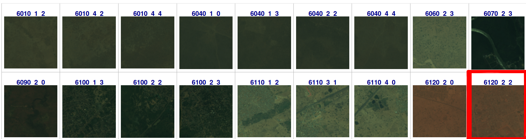
We do this for all the images of the training set and show the resulting images (from the R band tile).  These miniatures allow us to pick-up an interesting benchmark example that we can use for detailed studies.  In the following, we will use the image labeled 6120_2_2.  It shows a village in a dusty desert.

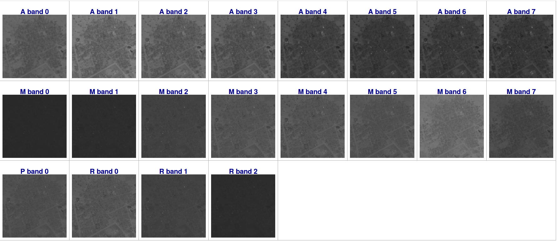
For the selected image, we can show the intensity of each spectral band.  We can immediately see that each spectral band contains complementary information of the same geographical location.  

From this step, it’s already obvious that we can exploit the difference of the band intensity to categorize objects on the ground.

3) Object Polygons

For the images in the training set, DSTL/Kaggle also provides GeoJSON files indicating the location of identified objects on the ground.  The JSON files contain coordinates of polygon vertices associated with the objects of a given class type.  

The files are easily loaded thanks to Geotrellis (GeoJson.fromFile) functions.  The library also offers functions to make a raster image out of the vectorial polygon information.  We use the function “PolygonRasterizer.foreachCellByPolygon” to create masks of the various object class types visible on the images.  

The image grid_sizes are used in this process in order to project the vectorial polygons on the raster images.  

In the figure below, identified objects are shown as black pixels.

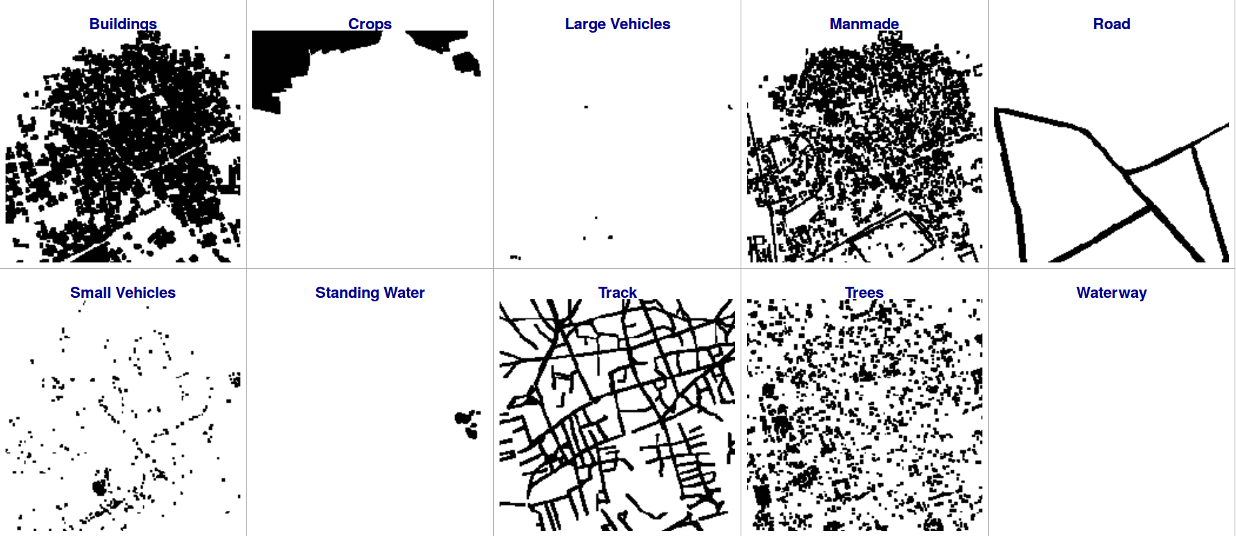
We can use those masks to select pixels associated to specific object class types from the 20 available spectral bands.  These pixels will be used to build a machine learning algorithm trained to identify specific objects.  

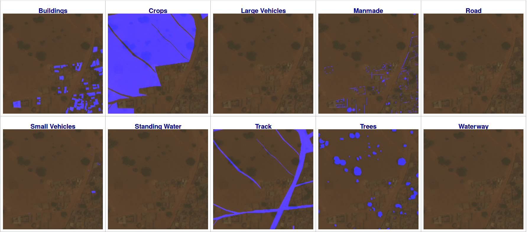
Before that, we will zoom in the top-left corner of the picture and overlay (in blue) the object polygons to the RGB picture in order to observe the level of details of the polygons (and of the picture).  We can also observe that some pixels belong to more than one object class.  Note for instance that the “trees” in the left part of the pictures are also part of a “crop”.  The prediction algorithm that we are designing will, therefore, need to achieve multi-class tagging with the same level of details than what we see here.

4) Spectral Histograms per object types

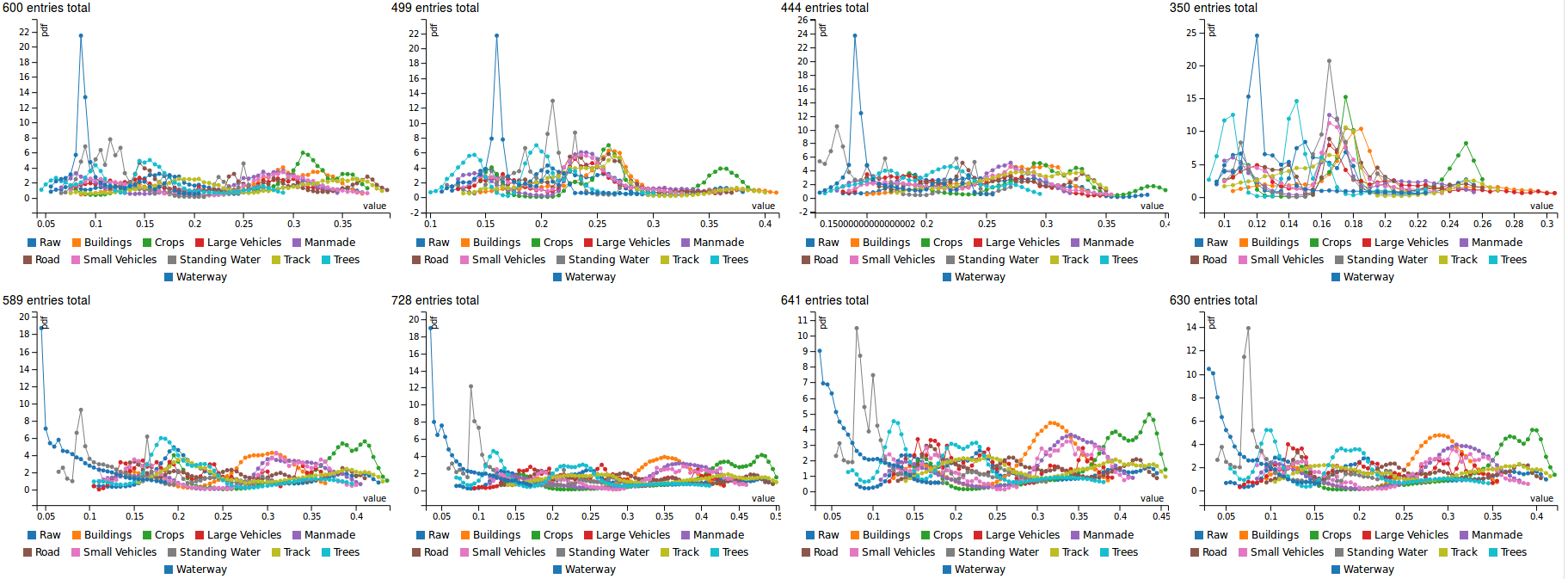
At this stage, it is interesting to see how the raw image histogram (per spectral band) by the object type masks.  This tells us which bands are useful to discriminate some object types.  

For instance, We see that the near-IR2 band is particularly good at discriminating water, building, and crops from the rest.  Other bands might be more performant for other objects.

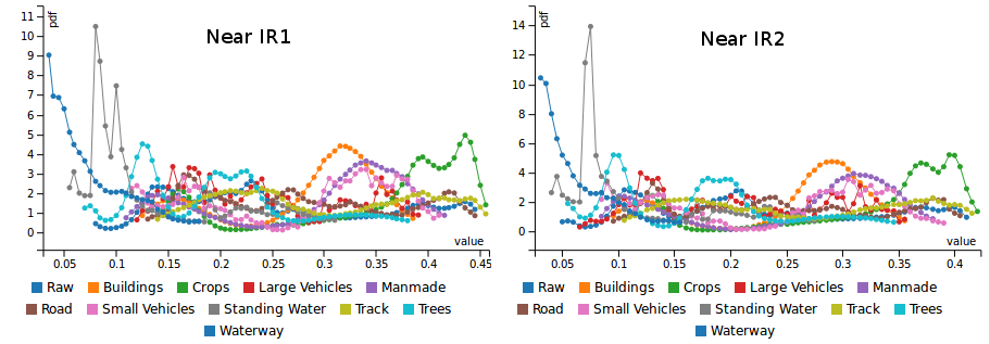
The figure below shows the histogram for the 8 bands of the ‘M’ GeoTIFF

5) Model Learning

We will H2O Sparkling-Water to train Gradient Boosted Machine (GBM) models that discriminate pixels of one object class type from the rest, using a one-vs-all approach.  As we have 10 possible class types, we train 10 different algorithms returning the probability that a pixel belongs to a given class type.  

Note:  Other approaches might lead to better performances at the cost of higher code complexity and training time.

To train the algorithms on class type, we create a dataset made of 200K randomly chosen pixels belonging to the class type and of 200K pixels not belong to it.  For each pixel, we collect the intensity of the 3+1+8+8 spectral bands. This dataset is converted into an H2O Frame and split into a training dataset (90%) used to train the GBM algorithm and a validation dataset (10%) that is used to evaluate the performance of the trained algorithm to identify object type of the pixels.  

The training is distributed on a Spark cluster via Sparkling-Water.  The GBM is made of 100 trees with a maximal depth of 15.  

The performance of the model is obtained from the Area Under Curve (AUC) computed on the validation dataset.  The AUC is at best equal to 1.0 and a model is generally considered satisfactory when it has an AUC above 0.8.  The operation is repeated for each class type.  The table below summarizes the model AUC of each object class type.

Object Type	Model AUC
Buildings	0.992441
Manmade	0.966026
Road	0.997235
Track	0.930540
Trees	0.960790
Crops	0.983181
Waterway	0.999718
Standing Water	0.999889
Large Vehicles	0.999354
Small Vehicles	0.997031

The trained models are saved in the form of MOJO files which we could easily import in Scala/Java when we’ll want to use them.

6) Pixel Clustering and Model Prediction

The previous section closed the model learning part of this analysis.  In the next sections, we will use the trained model to identify the objects on raw pictures (for which we don’t have the polygons).

Note: for comparison purposes, we keep using the image labeled 6120_2_2 as the benchmark example.

Running the model prediction on the 11.5M pixels of the 450 images of the dataset is extremely time-consuming.  

Hint: because many pixels on each picture have very similar spectral intensity, we can save a lot of computing time by clustering similar neighboring clusters together and compute the model prediction at the level of the pixel cluster.  

We develop a simple algorithm to aggregate adjacent clusters which have similar spectral information (with a tolerance of 3%).  The cluster color is taken as the color average of the constituting pixels.  In a second stage, small clusters (<50 pixels) are merged with the surrounding cluster with the closest color.  

Finally, the previously trained models are used to predict the probability that an entire cluster belong to each of the 10 possible object class types.

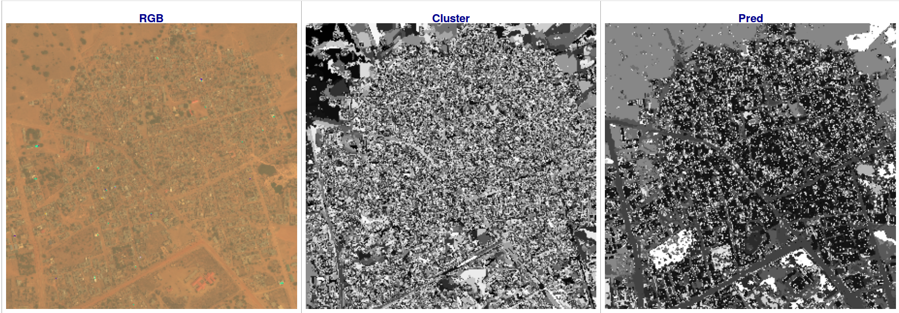
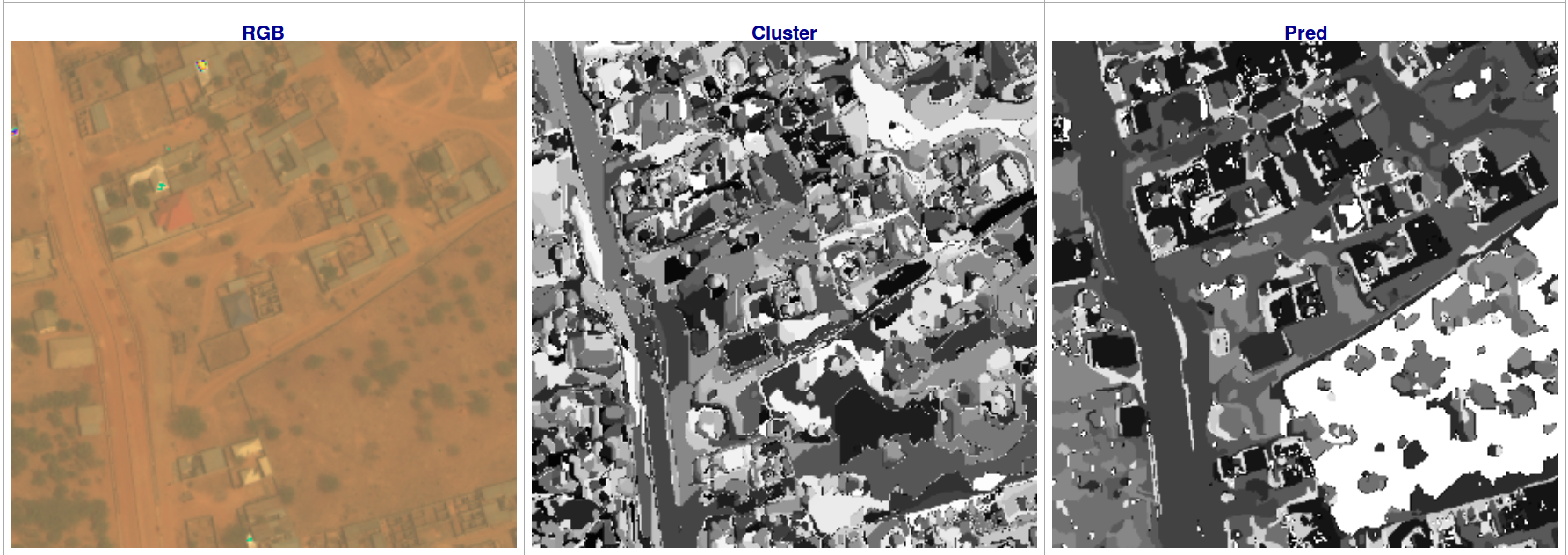
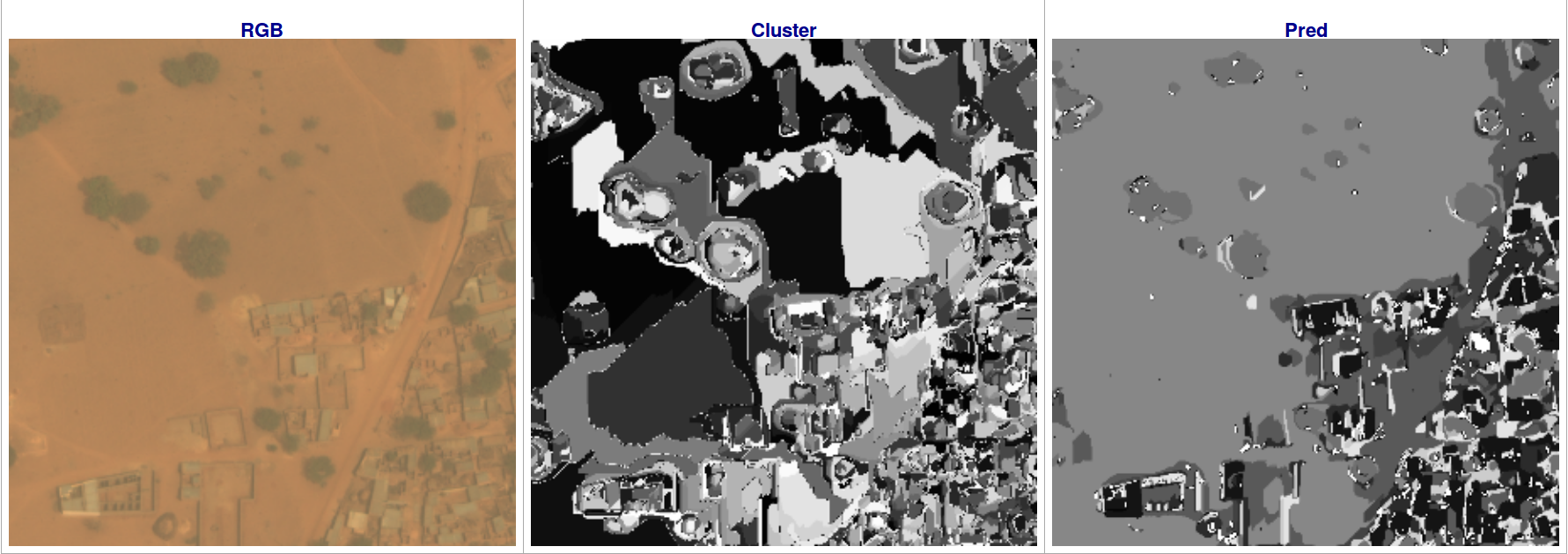
The result of this algorithm is shown below for the 6120_2_2 image. The first row, shows the full image, while the middle and bottom rows are zoomed in the bottom-left and on the top-left corner of the image respectively.  The three columns show, from left to right:

• The R-band image: the image brightness was increased to better appreciate the objects on the image.  This results in some (harmless) color glitches in the overexposed area.
• The identified clusters on the image.  Where the cluster are randomly colored using a 256 gray levels palette.  In other words, color has no particular meaning here.
• The identified clusters on the image colored according to the most probable class type of the object belonging to the cluster.  An eleventh color level is also present for clusters belonging to none of the object class types.  On these pictures, we can see that the shape of the objects in the picture is quite visible.

7) Mask Predictions

From this information, we can create a raster mask per object class type indicating the presence of an object or not.  Overlap of object class types is handled by a set of ad hoc rules based on other class types probability for this cluster and for the surrounding ones.  

Example, we know that the chances to find a truck in the middle of a waterway area are null.  Similarly, having a tree on top of a road is unlikely.  On the contrary, finding a car or a truck on a road is quite probable, so as finding a tree in the middle of a crop.

These rules are tuned by hand based on what is observed in the training dataset.  More sophisticated rules taking, for instance, into account the size of the cluster could also be added.  Having a crop cluster made of a few pixel or a car of thousands of pixels are both quite unlikely.  But we didn’t push the exercise that far for this blog.
We overlay in blue the masks that we obtained on the bottom-left corner of R-band image.  These predicted masks are directly comparable with those shown in section 3).  From this, we can see that we are doing quite well for identifying Building, Crops, and Trees.  For Manmade structures, and vehicles we overpredict quite a bit.  And our algorithms has a hard time to make difference between road and tracks in this dusty environment.  

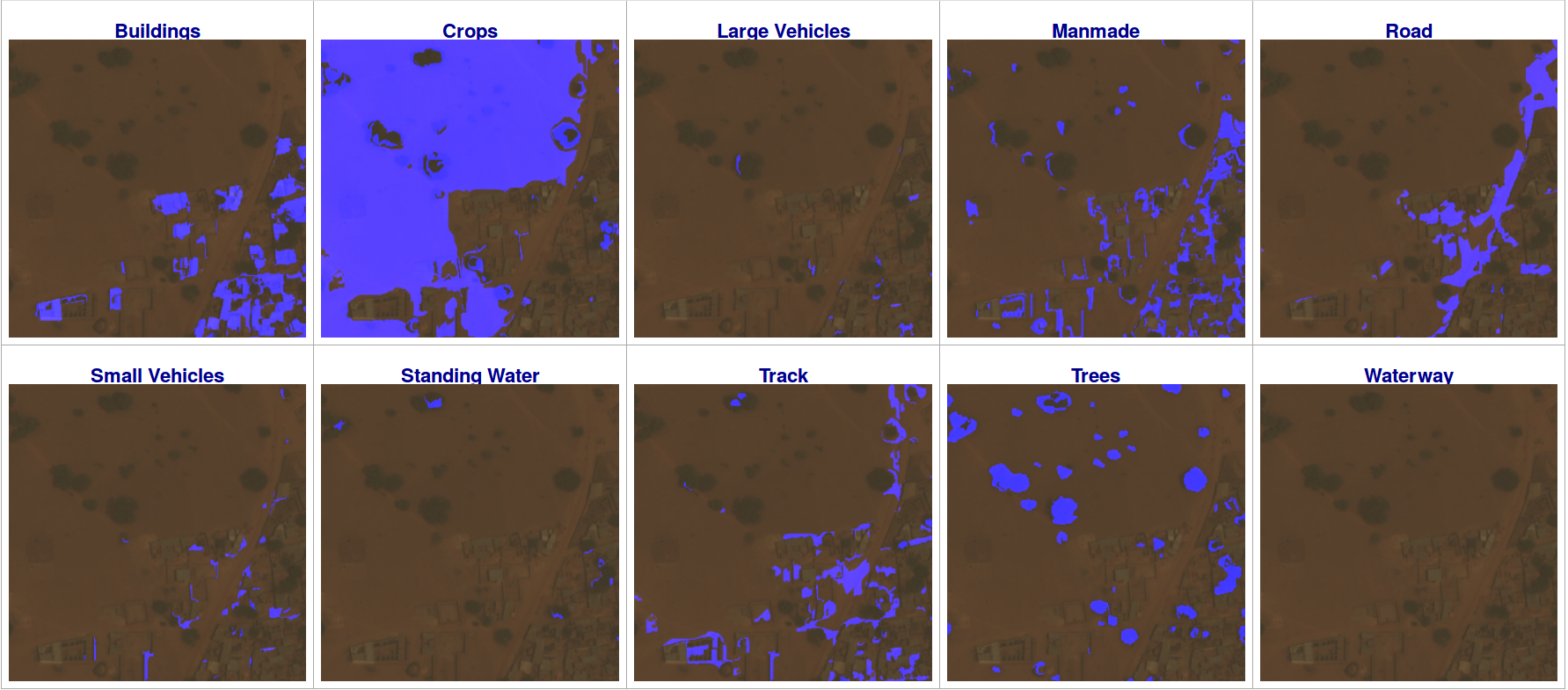
These issues could be solved by implementing more complex rules for the class overlaps (as discussed earlier) and/or by completing the one-vs-all models by some dedicated one-vs-one models which could be used to solve the ambiguities between road vs tracks, large vs small vehicles or standing water vs waterway.  Again, we didn’t push the exercise that far for this introductory blog.

8) Mask Vectorizing

In this last step, we convert the object raster masks into a list of polygons.  The Geotrellis Tile.toVector function allows doing this quite easily.   The image grid_sizes are used in this process in order to translate pixel coordinates into vectorial coordinates on the grid.

We notice that for complex rasters with holes (i.e. the mask of the crops shown above), the function may have difficulties in identifying the underlying polygons.  In this case, we split the raster in 4 quarters and try to vectorize each of the quarters separately.  This procedure is applied iteratively until the sub-quarter rasters get to small or the vectorizer succeeds at identifying the polygons.

Geotrellis also provides high-level functions to manipulate/modify the polygons.  We can, for instance, simplify the polygons to make them smoother and reduce their memory/disk footprint.

Finally, the polygons are saved on disk either in GeoJSON format or in WKT format.

Summary

We have shown how to combine the Spark, Geotrellis, H2O Sparkling-Water and the Spark-Notebook to perform scalable geospatial data analysis.  We’ve taken an end-to-end benchmark example involving distributed Extract-Transform-Load (ETL) on GeoTIFF and GeoJSON data, Multi-spectral geospatial images analysis, a pixel based object tagger training, and more.

If you like this blog and are eager to see more details on this GIS benchmark, you should have a look at this example repository.  Remember that all these notebooks are in read-only mode, so you can only see them.  If you want to play with your own example you gonna have to take the 5 min needed to install the Spark-Notebook on your machine. 

 

 

 

 

 

Have you already faced similar type of issues ?  Feel free to contact us, we'd love talking to you…

If you enjoyed reading this post, please like it. It doesn't cost you anything, but matters for me!